
Avian Physics 0.4 has been released! 🪶
Avian is an ECS-based 2D and 3D physics engine for Bevy, a refreshingly simple data-driven game engine built in Rust. Avian prioritizes ergonomics and modularity, with a focus on providing a native ECS-driven user experience.
Check out the GitHub repository and the introductory post for more details.
Highlights
Avian 0.4 is the biggest release yet, with several new features, quality-of-life improvements, and important bug fixes. Highlights include:
- Massive performance improvements: Avian is 3x as fast as before, with much better scaling for multi-core hardware.
- Solver bodies: The solver stores bodies in a much more efficient format optimized for cache locality and future wide SIMD support.
- Graph coloring: The constraint solver is now multi-threaded with graph coloring.
- Simulation islands: Islands are used for a much improved sleeping and waking system, reducing overhead for large game worlds with many resting bodies.
- Force overhaul: The force and impulse APIs have been redesigned from the ground up, providing a much more capable and intuitive interface.
- Joint improvements: Joints now support full reference frames (anchor + basis), and have new
JointDampingandJointForcescomponents. - Voxel colliders: Avian now supports voxel colliders for efficient representation of Minecraft-like worlds and other volumetric data.
- Bevy 0.17 support: Avian has been updated to the latest version of Bevy, and has changed its collision event types and system set naming to match.
- Contact API improvements: Contact data now provides access to world-space points, normal speeds, and more accurate contact impulses.
- Benchmarking CLI: Avian has a new CLI tool for benchmarking various scenes and profiling multi-threaded scaling.
The migration guide and a more complete changelog can be found on GitHub.
Performance Improvements
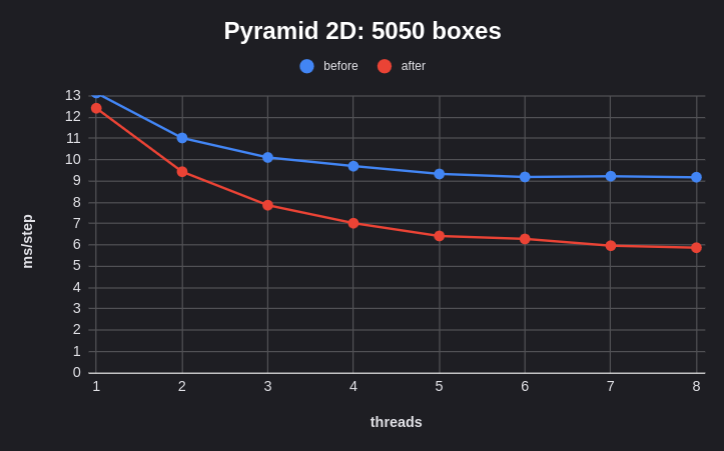
Avian 0.4 is approximately 3x as fast as Avian 0.3, with much better scaling for multi-core hardware.
CPU: Core i7-13700F
Getting to this point involved several changes and improvements to the solver, the largest of which are described below.
We will dive rather deep into how everything works, so if you just want to read about user-facing changes in Avian 0.4, feel free to skip ahead to the Force Overhaul section.
Solver Bodies
In past releases, our solver was highly bottlenecked by expensive ECS queries and sub-optimal cache performance.
Each constraint used a horribly inefficient RigidBodyQuery for the involved bodies, fetching 21 different properties/components,
many of which are optional. This resulted in a ton of overhead in a very hot loop.
For the curious: the RigidBodyQuery type in Avian 0.3
Uh… Yikes!
#[derive(QueryData)]
#[query_data(mutable)]
pub struct RigidBodyQuery {
    pub entity: Entity,
    pub rb: Ref<'static, RigidBody>,
    pub position: &'static mut Position,
    pub rotation: &'static mut Rotation,
    pub previous_rotation: &'static mut PreviousRotation,
    pub accumulated_translation: &'static mut AccumulatedTranslation,
    pub linear_velocity: &'static mut LinearVelocity,
    pub(crate) pre_solve_linear_velocity: &'static mut PreSolveLinearVelocity,
    pub angular_velocity: &'static mut AngularVelocity,
    pub(crate) pre_solve_angular_velocity: &'static mut PreSolveAngularVelocity,
    pub mass: &'static mut ComputedMass,
    pub angular_inertia: &'static mut ComputedAngularInertia,
    #[cfg(feature = "3d")]
    pub global_angular_inertia: &'static mut GlobalAngularInertia,
    pub center_of_mass: &'static mut ComputedCenterOfMass,
    pub friction: Option<&'static Friction>,
    pub restitution: Option<&'static Restitution>,
    pub locked_axes: Option<&'static LockedAxes>,
    pub dominance: Option<&'static Dominance>,
    pub time_sleeping: Option<&'static mut TimeSleeping>,
    pub is_sleeping: Has<Sleeping>,
    pub is_sensor: Has<Sensor>,
}
Avian 0.4 refactors the solver internals to use dedicated SolverBody and SolverBodyInertia types
optimized for memory locality and performance. They are initialized with body data before the solver,
and the results are written back after the solver. In 2D, the types currently look like this:
// This representation is inspired by b2BodyState in Box2D v3.
// 32 bytes in 2D, 56 bytes in 3D
#[cfg(feature = "2d")]
pub struct SolverBody {
    pub linear_velocity: Vec2,  // 8 bytes
    pub angular_velocity: f32,  // 4 bytes
    pub delta_position: Vec2,   // 8 bytes
    pub delta_rotation: Rot2,   // 8 bytes
    pub flags: SolverBodyFlags, // 4 bytes
}

// This representation is my own current design.
// 16 bytes in 2D, 32 bytes in 3D
#[cfg(feature = "2d")]
pub struct SolverBodyInertia {
    // Includes locked axes
    effective_inv_mass: Vec2,   // 8 bytes
    effective_inv_inertia: f32, // 4 bytes
    dominance: i16,             // 2 bytes
    flags: InertiaFlags,        // 2 bytes
}
Only awake dynamic bodies and kinematic bodies have an associated solver body. Static bodies and sleeping dynamic bodies
do not move, so they instead use a “dummy state” with SolverBody::default(). However, this raises a problem:
if the solver doesn’t have access to the position or rotation of static bodies, how can we compute constraint anchors?
There are two options:
- Option 1: Use delta positions and rotations. This requires preparing base anchors and other necessary positional data in world space, and computing the updated anchors during substeps.
- Option 2: Use full positions and rotations. This requires storing anchors in world space for static bodies and sleeping bodies, and in local space for dynamic bodies.
Avian uses Option 1, because:
- Using delta positions reduces round-off error when bodies are far from the origin.
- Mixing world space and local space values depending on the body type would be quite confusing and error-prone, and would possibly require more branching.
This required some refactoring for constraints, namely to prepare the base rotational data and to change some more logic to work in terms of deltas.
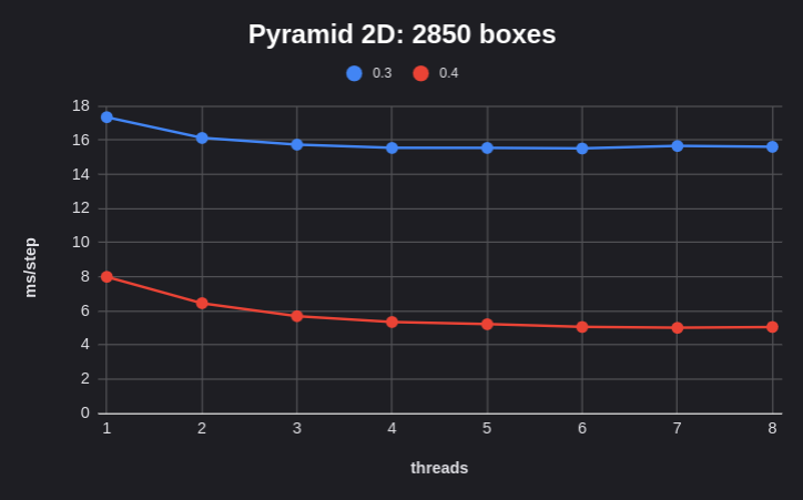
The results after switching to solver bodies are quite remarkable. In the pyramid_2d example, using a base of 75 boxes,
the results look like the following with 4 substeps and the parallel feature enabled.
CPU: Core i7-13700F
That is nearly a 3x performance improvement in this collision-heavy scene. Crazy!
Parallel Solver With Graph Coloring
Adding solver bodies was a massive performance improvement. However, the constraint solver was still entirely single-threaded, which imposed a fundamental limitation on how the simulation scales on multi-core hardware.
Parallelizing the solver is a non-trivial problem. Most physics engines, including Avian, use a Gauss-Seidel solver, which in practice means that constraints are solved sequentially, applying impulses to the bodies in a serial manner. To parallelize such a solver without race conditions, we need to identify sets of constraints that do not access the same bodies.
Roughly speaking, there are two or three common approaches to achieve this:
- Simulation islands: Bodies are grouped into graph-like “islands” based on their constraints. Islands are disjoint, so they can be simulated independently and in parallel.
- Graph coloring: Constraints are assigned to “colors” such that no adjacent constraints in the constraint graph share the same color. This ensures that each body can only appear once in each color, and all constraints within a given color can be solved in parallel.
- Hybrid: Islands are used as a coarse parallelization unit, and large islands can be further split with some algorithm similar to graph coloring.
Option 1 is fairly simple, but breaks down with large islands, as all constraints within a given island must still be solved serially. Option 2 is theoretically very effective, but the global graph coloring step itself can be costly. Option 3 is kind of a mix of both, only using graph coloring for large islands that need it.
Avian 0.4 implements a parallel constraint solver with graph coloring (option 2). To minimize overhead, the coloring is persisted across time steps, and updated incrementally using a simple greedy algorithm. This makes global graph coloring feasible even for huge worlds with tens of thousands of contacts.
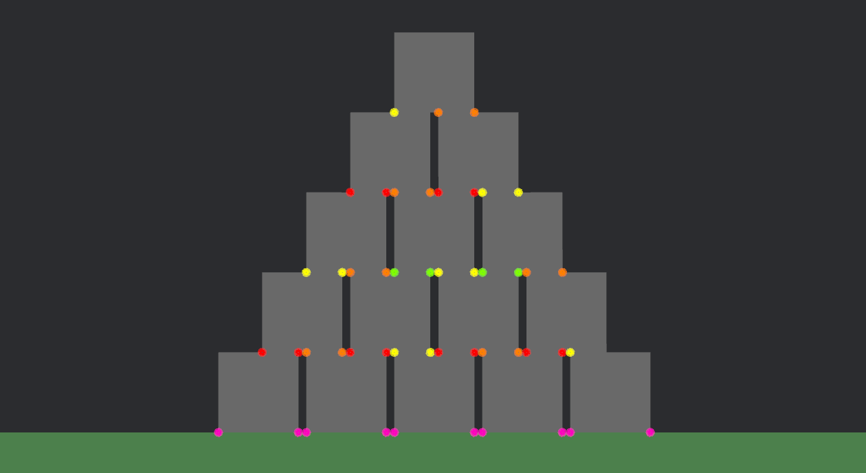
You can see it in action below. Each contact constraint has one or more contact points with the same color. In this scene, there are five colors, and if you look at for example red, you can see that it only touches a box once per contact constraint. This is the secret sauce that allows solving multiple constraints simultaneously without race conditions.
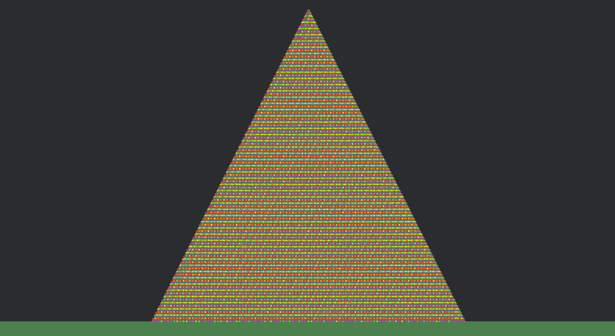
Scaling to a larger scene, it looks like this:
The next section describes the implementation. If you want to skip ahead, the performance results are shown in the Results section.
Implementation
The graph coloring algorithm is based on Box2D and Erin Catto’s excellent SIMD Matters article, with the difference that Avian supports more than one manifold per contact pair, which means that a single contact pair’s manifolds can be split across several colors.
Firstly, the ConstraintGraph and GraphColor types look like this:
pub struct ConstraintGraph {
    pub colors: Vec<GraphColor>,
}

pub struct GraphColor {
    pub body_set: BitVec,
    pub manifold_handles: Vec<ContactManifoldHandle>,
    pub contact_constraints: Vec<ContactConstraint>,
    // TODO: Joints do not yet use graph coloring
}body_setstores a bit set where each bit corresponds to anEntityindex.manifold_handlesstores theContactIdand index of eachContactManifoldin this color.contact_constraintsstores all contact constraints that are a part of this color.
When a contact manifold is added to the constraint graph, the constraint is assigned to the first color where the bit set
does not have either body’s bit set to 1. Once the constraint has been assigned to a color, the body bits are set to 1.
This is a very fast operation.
impl ConstraintGraph {
    pub fn push_manifold(&mut self, contact: &mut ContactEdge) {
        // Initialize the color index to a serial "overflow" color,
        // in case no free color is found.
        let mut color_index = COLOR_OVERFLOW_INDEX;

        // Find the first free color.
        for i in 0..GRAPH_COLOR_COUNT {
            let color = &mut self.colors[i];

            if color.body_set.get(contact.body1) || color.body_set.get(contact.body2) {
                // Try the next color.
                continue;
            }

            // Free color found! Assign the bodies to it.
            color.body_set.set_and_grow(contact.body1);
            color.body_set.set_and_grow(contact.body2);
            color_index = i;
            break;
        }

        // Map the actual contact to the color (omitted)
    }
}
Handling static bodies
The actual implementation needs to consider static bodies separately. They do not need to be added to the graph, as they are not mutably accessed during the solver. Additionally, it is good to solve static contacts last to give them higher priority in the solver. The algorithm ends up looking roughly like this:
impl ConstraintGraph {
    pub fn push_manifold(&mut self, contact: &mut ContactEdge) {
        // Get whether the bodies are static (omitted)

        // Initialize the color index to a serial "overflow" color,
        // in case no free color is found.
        let mut color_index = COLOR_OVERFLOW_INDEX;

        if !is_static1 && !is_static2 {
            // Constraints involving only non-static bodies cannot be in colors reserved
            // for constraints involving static bodies. This helps reduce tunneling through
            // static geometry by solving static contacts last.
            for i in 0..DYNAMIC_COLOR_COUNT {
                let color = &mut self.colors[i];

                if color.body_set.get(contact.body1) || color.body_set.get(contact.body2) {
                    continue;
                }

                color.body_set.set_and_grow(contact.body1);
                color.body_set.set_and_grow(contact.body2);
                color_index = i;
                break;
            }
        } else if !is_static1 {
            // Build static colors from the end to give them higher priority.
            for i in (1..COLOR_OVERFLOW_INDEX).rev() {
                let color = &mut self.colors[i];

                if color.body_set.get(contact.body1) {
                    continue;
                }

                color.body_set.set_and_grow(contact.body1);
                color_index = i;
                break;
            }
        } else if !is_static2 {
            // Build static colors from the end to give them higher priority.
            for i in (1..COLOR_OVERFLOW_INDEX).rev() {
                let color = &mut self.colors[i];

                if color.body_set.get(contact.body2) {
                    continue;
                }

                color.body_set.set_and_grow(contact.body2);
                color_index = i;
                break;
            }
        }

        // Map the actual contact to the color (omitted)
    }
}
Similarly, when a contact manifold is removed from the constraint graph, the corresponding bits are cleared in the bit set.
impl ConstraintGraph {
    pub fn pop_manifold(&mut self, contact: &mut ContactEdge) -> Option<ContactConstraintHandle> {
        // Pop the constraint handle mapping the contact to this color.
        let constraint_handle = contact.constraint_handles.pop()?;

        // Get the constraint's color and the index within that color.
        let color_index = constraint_handle.color_index;
        let local_index = constraint_handle.local_index;
        let color = &mut self.colors[color_index];

        if color_index != COLOR_OVERFLOW_INDEX {
            // Remove the bodies from the color's body set.
            color.body_set.unset(contact.body1);
            color.body_set.unset(contact.body2);
        }

        // Remove the manifold handle from the color (omitted)

        // Return the constraint handle that was removed.
        Some(contact_constraint_handle)
    }
}Now, the solver can simply iterate through each color, and solve the constraints in a given color in parallel.
Under the hood, implementing the constraint graph and graph coloring involved a lot more changes:
- The
ContactGraphnow storesContactEdges (“cold” connectivity data) andContactPairs (the actual contact data) separately - The
ContactGraphnow usesIdPools to keepContactEdgeindices stable when contacts are added or removed - Active and sleeping
ContactPairs are now stored in separate lists, allowing the narrow phase to only iterate over active contacts ContactConstraintpreparation is now done in the solver, not in the narrow phase- A lot more :)
Results
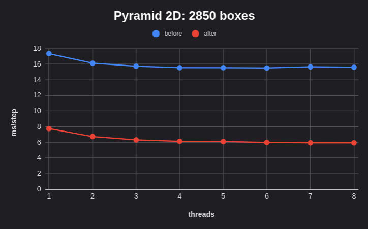
Running the Large Pyramid 2D benchmark before and after implementing graph coloring, we get the following results:
CPU: Core i7-13700F
A more detailed breakdown can be seen below. Before graph coloring:
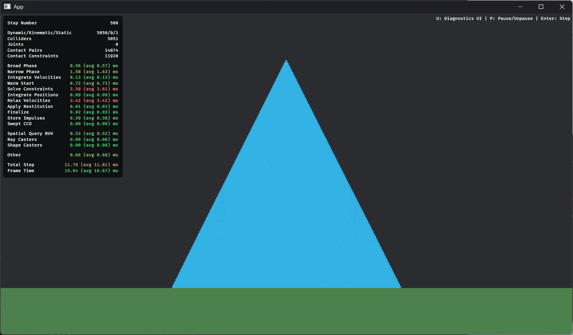
After graph coloring:
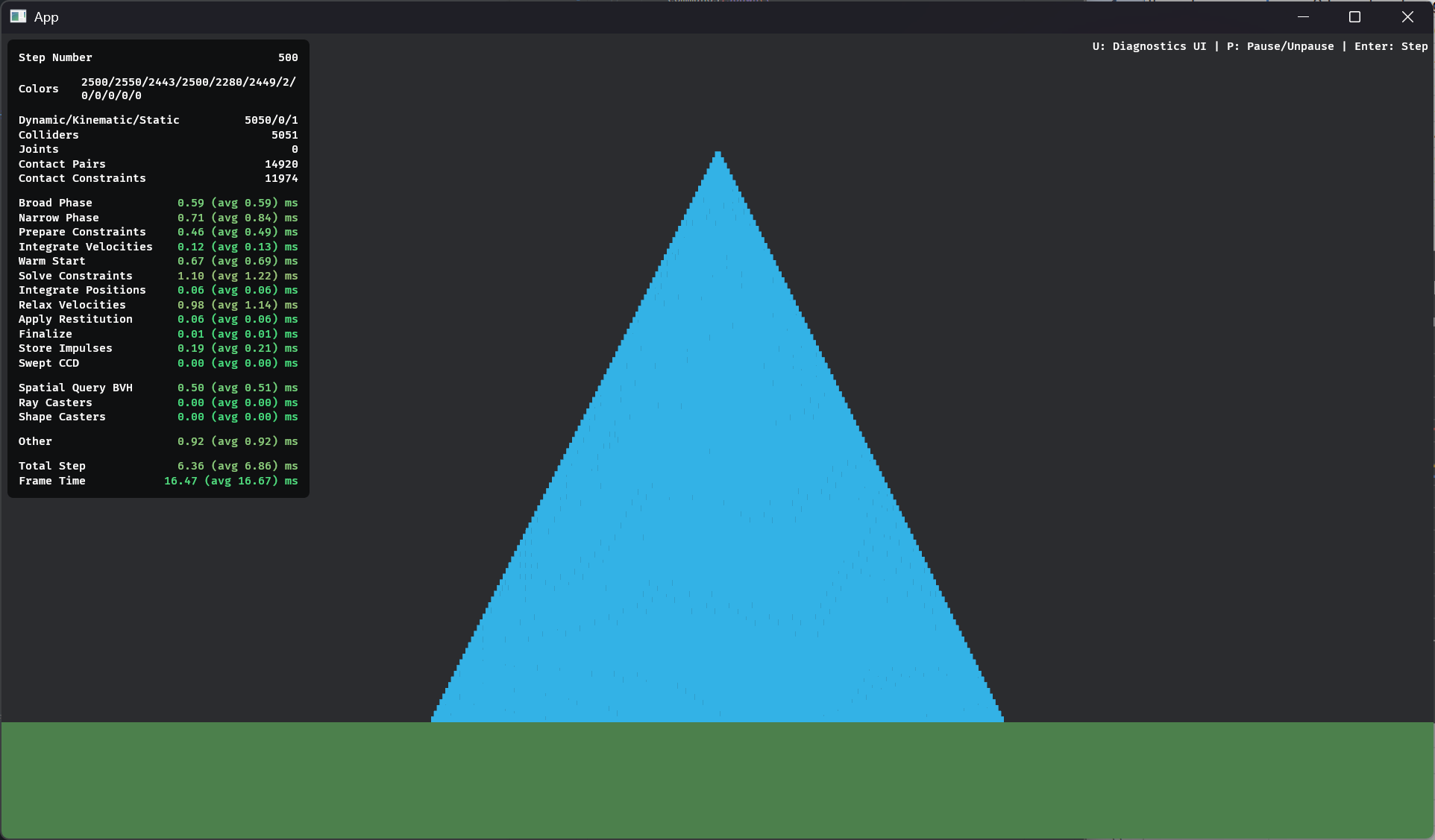
At the top of the profile you can see the contacts being assigned to graph colors. You can see how the narrow phase is now significantly faster, and more importantly the solver is over 3x as fast, resulting in nearly 2x total performance. This difference tends to grow the more contacts there are.
This is just the start, as there is a lot more that can be done to further optimize things:
- The threading should be optimized further to minimize latency and effectively go as wide as possible, as fast as possible. See the Improved Multi-Threading section at the end.
- Graph coloring is not just for multi-threading; it also enables AoSoA-style SIMD optimizations. See the Wide SIMD section at the end.
- Joints do not use graph coloring just yet, but it should be relatively straightforward to add support for it soon.
Expect more improvements in the future!
Simulation Islands
In the previous section, simulation islands were mentioned as one approach for solver parallelization. However, they also have another, arguably even more important function: sleeping and waking!
Sleeping is a low-cost state for resting dynamic bodies, and it is crucial for reducing CPU overhead for large game worlds. Up until now, Avian has used basic per-body sleeping that only allows sleeping for dynamic bodies that are not in contact with each other and not connected via joints. This meant that object piles and joints were never allowed to sleep.
The standard solution to this problem is simulation islands. Bodies that are touching or connected by a joint belong to the same island, and can only sleep if the whole island can sleep. Conversely, if any dynamic body in an island is woken up, the whole island is woken up.
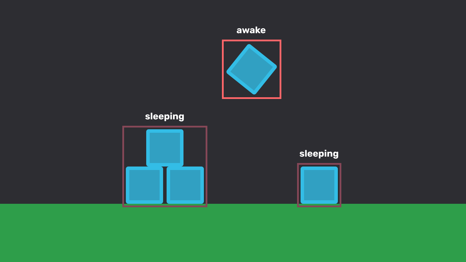
Avian 0.4 implements persistent simulation islands for sleeping and waking. Islands are persisted across time steps, merged when constraints are added between different islands, and split heuristically in a deferred manner.
This can be seen in action in the below video, displaying the combined bounds of each body in each island as a red bounding box. When islands are marked as sleeping, the outline becomes darker.
Implementation
The island implementation is primarily based on Erin Catto’s Simulation Islands article and Box2D. In short:
- Each dynamic body starts with its own
PhysicsIsland, stored in thePhysicsIslandsresource. - Bodies, contacts, and joints form island linked lists with an
IslandNodestored in eachBodyIslandNodecomponent,ContactEdge, andJointEdge. - When a constraint between two dynamic bodies is created, their islands are merged with a serial union-find algorithm.
- When a constraint is removed,
PhysicsIsland::constraints_removedis incremented. - At each time step, the sleepiest island with one or more constraints removed is chosen as a
split_candidate, and split using DFS. Splitting is expensive, but it can safely be deferred and done heuristically like this.
For more details, see #809.
The persistent approach is extremely fast, as shown in Erin’s article. Of course, a downside is that it needs to persist state, which can complicate networking use cases. In the future, it could be worth also supporting a stateless alternative that builds islands from scratch for each time step using a depth-first search or union-find algorithm. In particular, Jolt uses a parallel union find algorithm that could be a solid alternative.
Force Overhaul
In past releases, the force APIs ExternalForce, ExternalTorque, ExternalImpulse, and ExternalAngularImpulse were quite limited and cumbersome to use. Everything could be “persistent” or “not persistent”, impulses were not applied immediately but rather during the simulation step, and local forces were not directly supported. Additionally, there was a lot of wasted memory, and overall inefficiencies.
Avian 0.4 overhauls the force APIs from the ground up, replacing the old components with two types of new APIs:
- Components for constant forces
- A
ForceshelperQueryData
Constant Forces
Constant forces and torques that persist across time steps can be applied using the following components:
ConstantForce: Applies a constant force in world space.ConstantTorque: Applies a constant torque in world space.ConstantLinearAcceleration: Applies a constant linear acceleration in world space.ConstantAngularAcceleration: Applies a constant angular acceleration in world space.
They also have local space equivalents:
ConstantLocalForce: Applies a constant force in local space.ConstantLocalTorque: Applies a constant torque in local space.ConstantLocalLinearAcceleration: Applies a constant linear acceleration in local space.ConstantLocalAngularAcceleration: Applies a constant angular acceleration in local space.
These components are useful for simulating continuously applied forces that are expected to remain the same across time steps, such as per-body gravity or force fields.
commands.spawn((
    RigidBody::Dynamic,
    Collider::capsule(0.5, 1.0),
    // Apply a constant force of 10 N in the positive Y direction.
    ConstantForce::new(0.0, 10.0, 0.0),
));
The forces are only constant in the sense that they persist across time steps. They can still be modified in systems like normal.
Forces Helper
It is common to apply many individual forces and impulses to dynamic rigid bodies, and to clear them afterwards. This can be done using the Forces helper QueryData.
To use Forces, add it to a Query (without & or &mut), and use the associated methods to apply forces, impulses, and accelerations to the rigid bodies.
fn apply_forces(mut query: Query<Forces>) {
    for mut forces in &mut query {
        // Apply a force of 10 N in the positive Y direction to the entity.
        forces.apply_force(Vec3::new(0.0, 10.0, 0.0));
    }
}
The force is applied continuously during the physics step, and cleared automatically after the step is complete.
Forces can also apply forces and impulses at a specific point in the world. If the point is not aligned with the global center of mass, it will also apply a torque to the body.
// Apply an impulse at a specific point in the world.
// Unlike forces, impulses are applied immediately to the velocity,
forces.apply_linear_impulse_at_point(force, point);
As an example, you could implement radial gravity that pulls rigid bodies towards the world origin with a system like the following:
fn radial_gravity(mut query: Query<(Forces, &GlobalTransform)>) {
    for (mut forces, global_transform) in &mut query {
        // Compute the direction towards the center of the world.
        let direction = -global_transform.translation().normalize_or_zero();
        // Apply a linear acceleration of 9.81 m/s² towards the center of the world.
        forces.apply_linear_acceleration(direction * 9.81);
    }
}
By default, applying forces to sleeping bodies will wake them up. To avoid this, call non_waking to get a non-waking instance of the force item.
// This does not wake the body up.
forces.non_waking().apply_force(force);

// This wakes up the body if it is sleeping.
forces.apply_force(force);
Joint Improvements
For a long time, Avian’s joints have been in dire need of a rework. While the new joint solver is unfortunately still not ready, I wanted to address some of the bigger API problems and missing features in this release.
Avian 0.4 implements:
- Reference frames (anchor + basis)
- Controlling damping via a
JointDampingcomponent - Accessing joint forces via a
JointForcescomponent - Disabling collisions between jointed bodies via a
JointCollisionDisabledcomponent - Querying for joints between entities through a
JointGraph - Decoupling joint APIs from solver internals, making custom joint solvers more viable
- A lot of polish to both APIs and documentation
Future work still includes the new joint solver, more joint types, and joint motors, to name a few. Still, progress has been made!
The following sections cover the above improvements in more detail.
Reference Frames
A very common problem that users have encountered with joints is that you can only configure the joint anchor’s position, but not the relative orientation. For a FixedJoint, this meant that the orientations of the two bodies were fixed to be equal, and you could not attach them together at a 45 degree angle, for example.
To address this, Avian 0.4 adds support for full joint frames. To illustrate what this means, consider the following image:

Each joint has two reference frames formed by an “anchor” and “basis”, one for each body. The anchor is the joint’s attachment point relative to the center of the body, while the basis is the joint’s base rotation relative to the orientation of the body. When these two reference frames are aligned in world space, such as in the illustration above, the translational and rotational offset between the bodies is considered to be zero.
Simply put, joint frames allow configuring the base translational and rotational offset for each body connected by a joint. By default, the offsets are zero, but they can be modified to achieve desired joint configurations.
In code, this is done with a JointFrame that contains a JointAnchor and JointBasis. They are enums with Local and FromGlobal variants, allowing the initialization of local frames using world-space values:
// Use a world-space anchor of (5, 2), and rotate the second body's local frame by 45 degrees.
commands.spawn((
    RevoluteJoint::new(body1, body2)
        .with_anchor(Vec2::new(5.0, 2.0))
        .with_local_basis2(Rot2::degrees(45.0))
));Damping
Previously, each joint type stored its own damping coefficients. However, the actual damping logic is not joint-specific, and not all joints need damping. Thus, it is now handled by a separate JointDamping component with linear and angular properties.
commands.spawn((
    DistanceJoint::new(body1, body2),
    JointDamping {
        linear: 0.1,  // Linear damping
        angular: 0.1, // Angular damping
    },
));
Forces
The details of joint forces are solver-specific. However, ultimately users want to read a force and torque vector. This has now been generalized as a JointForces component that the constraint solver writes to and users can read. It is not added automatically and must be added manually for the desired joint entities.
commands.spawn((
    RevoluteJoint::new(body1, body2),
    JointForces::new(),
));
An example of where this may be useful is breaking joints when their forces or torques exceed some threshold:
fn break_joints(
    mut commands: Commands,
    query: Query<(Entity, &JointForces), Without<JointDisabled>>,
) {
    for (entity, joint_forces) in &query {
        if joint_forces.force().length() > BREAK_THRESHOLD {
            // Break the joint by adding the `JointDisabled` component.
            // Alternatively, one could simply remove the joint component or despawn the entity.
            commands.entity(entity).insert(JointDisabled);
        }
    }
}
Disabling Joint Collision
A common requirement when using joints is to disable collisions between the attached bodies, for example a wheel and a car. Collision layers are typically not suitable for this, as you may still want a car to collide with the wheels of other cars.
In past releases, implementing the desired behavior properly required custom hooks, which is both inefficient and overly complicated for such a common scenario.
Avian 0.4 introduces a JointCollisionDisabled component for disabling collisions between bodies that are jointed together.
commands.spawn((
    RevoluteJoint::new(body1, body2),
    JointCollisionDisabled,
));
Joint Graph
To implement JointCollisionDisabled and simulation islands, it was necessary to have an efficient way to query for which bodies have joints between them. This naturally leads to a graph structure where bodies are nodes and the joints between them are edges.
Avian 0.4 adds a JointGraph resource for tracking how bodies are connected by joints. While it is primarily intended for internals, it can also be used as an API to query for whether two bodies are connected by a joint, or for querying all joints attached to a given body, without worrying about the types of joints involved.
Decoupling Solver Internals
Especially after refactoring constraint logic for solver bodies, the joint types stored a lot of data related to solver internals: Lagrange multipliers, center offsets from before the substepping loop, and more. This was not ideal. Such public APIs should not contain private internals, and it would also be good if these APIs could be reused even across different joint solvers, and were not inherently tied to our existing XPBD joint solver.
Avian 0.4 takes a big step towards a more decoupled design by moving solver-specific joint data into their own internal components like RevoluteJointSolverData, moving the joint APIs to a new dynamics::joints module, and extracting all XPBD logic into its own dynamics::solver::xpbd module with an XpbdSolverPlugin.
All XPBD logic is now gated behind an xpbd_joints feature, which means that (1) you can disable XPBD if you’re concerned about the patenting, and (2) it is now theoretically possible to implement your own custom solver for Avian’s joints, while using the existing API. Nice!
Voxel Colliders
Parry version 0.20 introduced a new Voxels
shape for efficiently representing 2D or 3D volumes made of small uniform cuboids, or voxels, commonly used for Minecraft-like terrain
or other volumetric data. The Voxels shape can offer improved performance and robustness due to its uniform structure, and notably,
it does not suffer from ghost collisions caused by internal edges.
Avian 0.4 uses the latest version of Parry, and adds support for voxel colliders.
You can see them in action for voxelized terrain in the voxels_3d example:
Voxel colliders can be created manually, or from a point cloud, or from a mesh. The following constructors are supported:
Collider::voxelsCollider::voxels_from_pointsCollider::voxelized_polyline(2D)Collider::voxelized_trimesh(3D)Collider::voxelized_trimesh_from_mesh(3D)Collider::voxelized_convex_decompositionCollider::voxelized_convex_decomposition_with_configCollider::voxelized_convex_decomposition_from_mesh(3D)ColliderConstructor::VoxelsColliderConstructor::VoxelizedPolyline(2D)ColliderConstructor::VoxelizedTrimesh(3D)ColliderConstructor::VoxelizedTrimeshFromMesh(3D)
Note that Parry’s current voxel implementation has some limitations:
- Collisions against composite shapes (ex: triangle meshes) are not yet supported.
- Debug assertions can sometimes cause crashes in debug mode, see parry#345.
Bevy 0.17 Support
Avian 0.4 supports Bevy 0.17, and includes changes to match its new conventions and APIs.
Collision Events
Bevy 0.17 introduced an Event / Observer Overhaul that changed how events work in Bevy. Notably, the new Message trait is what used to be a buffered Event, and Event is now left exclusively for observer events. Additionally, targeted events use the EntityEvent trait.
To adapt to these changes, Avian 0.4 combines its buffered events and observer events under the CollisionStart and CollisionEnd events. They implement both Message and Event, so they can be consumed with both the MessageReader and observer APIs, depending on which one is a better fit for a given scenario. This also means that the buffered events, or “messages”, now additionally store the entities of the bodies, not just the colliders.
Collision event terminology
The term “collision event” or “contact event” is extremely common across a variety of engines. With Bevy’s recent naming changes, it begs the question of whether we should abandon this standard and start calling the Message version a “collision message”.
From my point of view, the answer is no. The difference is subtle, but instead of saying that the type is a message, we say that it is written as a message. The defining factor of the type is that it is fundamentally a “collision event”, even if it can be sent as a message. See cart’s message on general naming guidelines for messages and events.
A collision event observer before and after:
// Before
fn on_player_stepped_on_plate(event: Trigger<OnCollisionStart>, player_query: Query<&Player>) {
    let pressure_plate = event.target();
    let other_entity = event.collider;

    if player_query.contains(other_entity) {
        println!("Player {other_entity} stepped on pressure plate {pressure_plate}");
    }
}

// After
fn on_player_stepped_on_plate(event: On<CollisionStart>, player_query: Query<&Player>) {
    let pressure_plate = event.collider1;
    let other_entity = event.collider2;

    if player_query.contains(other_entity) {
        println!("Player {other_entity} stepped on pressure plate {pressure_plate}");
    }
}
A collision event reader system before and after:
// Before
fn print_started_collisions(mut collision_reader: EventReader<CollisionStarted>) {
    for CollisionStarted(collider1, collider2) in collision_reader.read() {
        println!("{collider1} and {collider2} started colliding");
    }
}

// After
fn print_started_collisions(mut collision_reader: MessageReader<CollisionStart>) {
    // Note: The event now also stores `body1` and `body2`
    for event in collision_reader.read() {
        println!("{} and {} started colliding", event.collider1, event.collider2);
    }
}
System Sets
Bevy 0.17 adopted a consistent naming convention for system sets (I did this!). Where applicable, system sets should now be suffixed with Systems. Previously, Avian used the Set suffix, for example for PhysicsSet.
Avian 0.4 renames its system sets to follow the new Systems suffix convention. Notable renames include:
PhysicsSet→PhysicsSystemsPhysicsStepSet→PhysicsStepSystemsSubstepSet→SubstepSystemsSubstepSolverSet→SubstepSolverSystemsSolverSet→SolverSystemsIntegrationSet→IntegrationSystemsBroadPhaseSet→BroadPhaseSystemsNarrowPhaseSet→NarrowPhaseSystemsSweptCcdSet→SweptCcdSystemsPhysicsTransformSet→PhysicsTransformSystems
Collider Constructor Hierarchy Names
Bevy 0.17 changed the way Name works for glTF mesh primitives (migration guide). Instead of MeshName.PrimitiveIndex, it is now in the form of MeshName.MaterialName. This also means that APIs such as ColliderConstructorHierarchy::with_constructor_for_name have switched to this format.
ColliderConstructorHierarchy::new(ColliderConstructor::ConvexDecompositionFromMesh)
    .with_density_for_name("armL_mesh.ferris_material", 3.0)
    .with_density_for_name("armR_mesh.ferris_material", 3.0)
3D Friction Stability Fix
For a long time, Avian has had stability problems in 3D, especially with small shapes. Shapes with a small angular inertia drift and jitter on the ground even by themselves. A simple cube stack like the following with 10 cm cubes and the standard 9.81 m/s² gravity twists and just falls apart immediately.
As it turns out, this was a simple bug in the way tangent directions were computed for friction in the contact solver. In short, the “effective mass” for friction was computed using old tangents, but later substeps used new tangents while still using the original effective mass, which could produce wildly inaccurate impulses at low speeds where the tangents can change quickly. The fix was to instead just use the original tangents for the whole time step, not recomputing them each time.
With this fixed, we get a massive stability improvement:
There is still a small wobble, but I believe this is largely due to the gravity being fairly high for such small objects, and 6 substeps isn’t enough to keep it fully stable. With a lower gravity, it’s perfectly stable.
Contact API Improvements
Avian’s contact APIs have historically had some quirks that make them difficult to use. Avian 0.4 addresses some of these.
World-Space Points
In past releases, each ContactPoint stored a local_point1 and local_point2, the closest points between the surfaces of the two bodies in local space. However, users reading collision data typically only want a single point in world space to determine where the contact happened.
Avian 0.4 adds a ContactPoint::point property for the world-space contact point. This is effectively the midpoint between the closest points of the contact surfaces in world space. Additionally, the local contact points have been removed (for now) in favor of world-space anchor1 and anchor2 points relative to the center of mass of each body.
Contact Impulses
The impulse applied along the normal at a contact point is stored in the ContactPoint::normal_impulse property. However, in previous releases, this did not actually represent the total impulse applied over the whole time step, as it was instead the “clamped accumulated normal impulse” from the last substep. This representation was needed for warm starting the contact solver, but it did not match user expectations.
Avian 0.4 changes ContactPoint::normal_impulse to be the total impulse applied across the time step. The old warm starting impulse is now stored as ContactPoint::warm_start_normal_impulse. APIs such as ContactPair::total_normal_impulse have also been updated accordingly, to use the total impulse.
Additionally, each ContactPoint now exposes a normal_speed property for the relative velocity of the bodies along the normal. This can be thought of as an impact velocity: -normal_speed is equivalent to how fast the bodies are approaching each other at the contact point. This can be a useful alternative to normal_impulse for determining the “strength” of a contact in a way that is not dependent on mass or the time step.
Collider Constructor Caching
Generating colliders from meshes using ColliderConstructor or ColliderConstructorHierarchy can be expensive, especially when using convex decomposition. In past releases, each collider was always generated separately, but in practice, scenes tend to use many instances of the same meshes. Generating the same collider separately for each mesh instance can result in a lot of unnecessary work.
Avian 0.4 introduces caching for collider constructors. For each new mesh that needs a collider, the generated shape is added to a ColliderCache resource, and when a mesh with the same AssetId is encountered later, the shape is simply fetched from the cache rather than generating a new collider from scratch. This is enabled by default and requires no changes on the user’s side.
This can have a significant impact on scene loading times. Below, you can see how loading the Foxtrot scene used to take several seconds:
(Ignore the chair freaking out, that was an old bug that has since been fixed)
Now, loading the map is near instantaneous!
(the first load is a bit more costly here, and also included shader compilation, which is unrelated to Avian)
Collider Constructor Ready Events
There are cases where you may want to detect when a ColliderConstructor or ColliderConstructorHierarchy has finished generating its collider(s),
for example to delay logic that depends on the colliders being present. Doing this is a bit of a hassle and requires querying for the Collider.
Avian 0.4 adds some new events that aim to make the workflow easier.
ColliderConstructorReadyis triggered when aColliderConstructorhas successfully inserted aCollider.ColliderConstructorHierarchyReadyis triggered when aColliderConstructorHierarchyhas finished inserting all of itsColliders. It makes no guarantees about whether collider generation was successful for each entity.
Benchmarking CLI
With an increasing focus on performance and multi-threading, Avian needs better tooling for benchmarks. Version 0.3 added physics diagnostics, which are great for runtime profiling, but we are still missing a tool to simply run a suite of dedicated benchmarks that produce reliable, reproducible results in text form. Built-in Rust tooling like cargo bench and the criterion crate are not enough, as our needs are more specialized. We need tooling to:
- run benchmarks that track the desired physics timers, not just total step times
- run a benchmark with many different thread counts to profile multi-threaded scaling
- run a benchmark with different SIMD targets (AVX, SIMD128, NEON, SSE2, scalar)
- bonus: produce CSV files with the desired format to create plots for benchmark results
Avian 0.4 implements its own CLI tool for running 2D and 3D benchmarks. This is not a part of the crate itself, but can be found in the GitHub repository.
Currently, the CLI supports the following options:
Options:
  -n, --name <NAME>                The name or number of the benchmark to run. Leave empty to run all benchmarks
  -t, --threads <THREADS>          A range for which thread counts to run the benchmarks with. Can be specified as `start..end` (exclusive), `start..=end` (inclusive), or `start` [default: 1..13]
  -s, --steps <STEPS>              The number of steps to run for each benchmark [default: 300]
  -r, --repeat <REPEAT>            The number of times to repeat each benchmark. The results will be averaged over these repetitions [default: 5]
  -l, --list                       List all available benchmarks in a numbered list
  -o, --output <OUTPUT>            The output directory where results are written in CSV format. Leave empty to disable output
  -h, --help                       Print help
  -V, --version                    Print version
An example of running the “Large Pyramid 2D” benchmark with 1-6 threads and 500 steps, repeated 5 times:
# Run with `benches` as the current working directory
cargo run -- --name "Large Pyramid 2D" --threads 1..=6 --steps 500 --repeat 5
The output might look something like this:
Running benchmark 'Large Pyramid 2D' with threads ranging from 1 to 6:
| threads | avg time / step | min time / step |
| ------- | --------------- | --------------- |
|       1 |     12.29045 ms |     11.22260 ms |
|       2 |     10.40321 ms |      9.27592 ms |
|       3 |      9.65242 ms |      8.53754 ms |
|       4 |      9.19108 ms |      8.15204 ms |
|       5 |      9.03052 ms |      8.08754 ms |
|       6 |      8.91510 ms |      7.87406 ms |
The CLI supports CSV output, producing files like the following:
threads,step_ms
1,12.290453
2,10.403209
3,9.652423
4,9.191079
5,9.030517
6,8.915103
Creating plots (for example in Google Sheets or some other tool) is then very easy. You might have seen these earlier in this post!
In the future, when wide SIMD is used for the solver, we will also add different SIMD targets to the benchmarks. If we wanted to, we could also further automate plot creation by generating them directly as .png or .svg files in the CLI tool, but for now, they must be authored manually.
Other Changes and Fixes
There are still many, many other changes and fixes that I didn’t cover in detail in this post. Some notable ones include:
- Add
Collider::convex_polylineby @kirilllysenko in #727 - Improve CI performance and caching by @janhohenheim in #729, #730, #732, and #736
- Optimize gyroscopic motion by @Jondolf in #738
- Add
ColliderConstructor::Compoundby @Piefayth in #758 - Rework
PositionandRotationinitialization by @Jondolf in #760 - Fix
DistanceLimit::compute_correction()signs by @MiniaczQ in #766 - Upgrade to Rust 2024 edition by @Jondolf in #774
- Use
SymmetricMat3fromglam_matrix_extrasfor angular inertia by @Jondolf in #777 - Implement
DerefandIntoIteratorforRigidBodyCollidersby @Jondolf in #784 - Rework
SyncPlugin, removePreparePlugin, and improve scheduling by @Jondolf in #785 - Fix colliders not working after removing
Disabled/ColliderDisabledby @Jondolf in #791 - Fix
Plane3dcolliders ignoring half size by @janhohenheim in #795 - Add
tumblerexample by @Jondolf in #796 - Contact pruning for 3D by @Jondolf in #798
- Remove
rest_lengthfield fromDistanceJoint. by @shanecelis in #517 - Remove
countfromRayHitsandShapeHitsby @Jondolf in #808 - Add
ApplyPosToTransformcomponent @cBournhonesque in #837 - Show debug gizmos for interpolated transforms by @janhohenheim in #829
- Implement collider constructor ready events by @janhohenheim in #830
- Disable mass property warning for collider constructors by @Jondolf in #849
- Update collider scale when the shape changes, not just when the transform changes by @pcwalton in #851
- Don’t update the diagnostics UI if it isn’t visible by @pcwalton in #856
A more complete list of changes can be found on GitHub.
What’s Next?
Avian 0.4 is a massive step forward, but there is still a lot more to come. Here are some of the things I am looking to work on next!
Performance Improvements
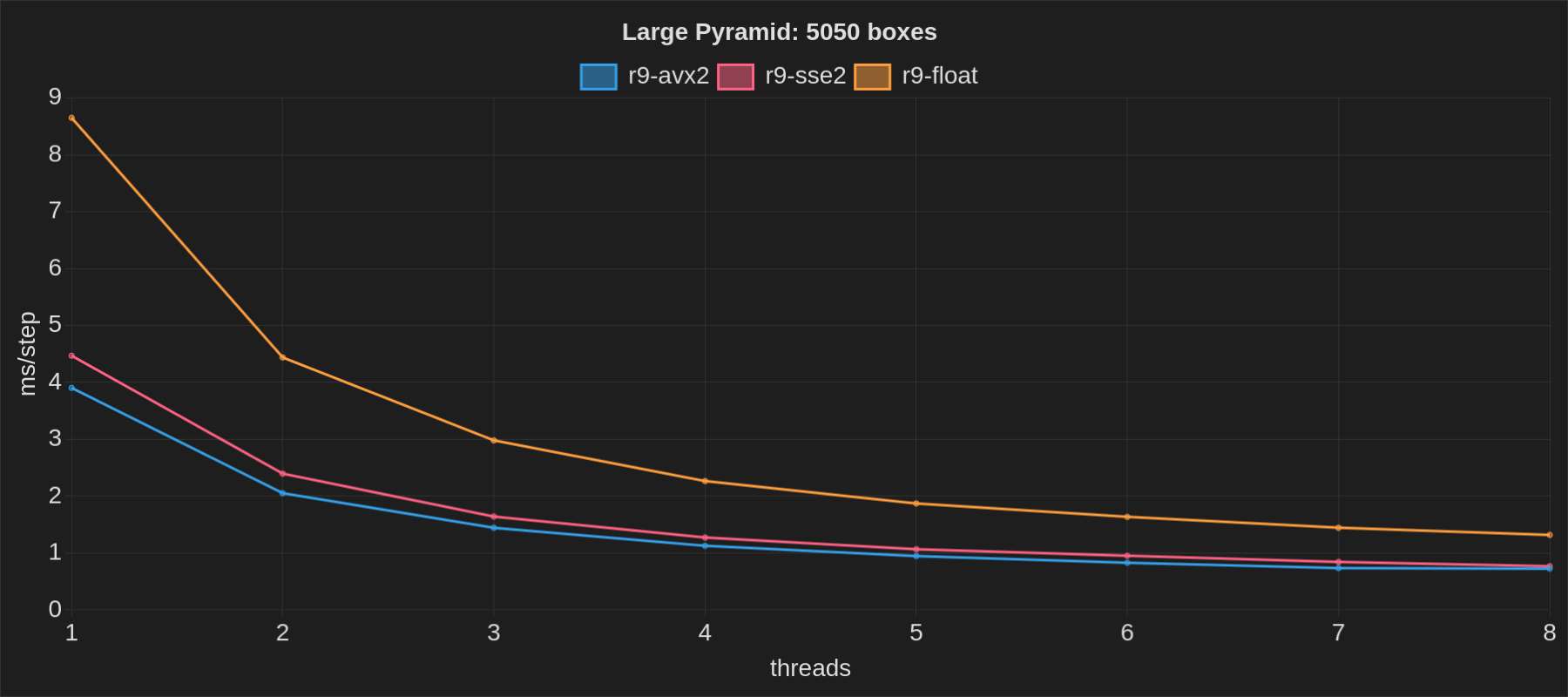
Wide SIMD
Earlier, we described how Avian 0.4 now uses graph coloring for multi-threading in the constraint solver. However, multi-threading is not the only form of parallelization. Modern CPUs also support various SIMD instructions for performing the same operation on multiple pieces of data at the same time, which can lead to significant performance gains for both single-threaded and multi-threaded use cases.
Leveraging SIMD properly is challenging, and requires the algorithm to be designed with vectorization in mind. While compilers can often perform auto-vectorization for appropriately formatted data, the best results can be achieved with manual vectorization. To give an idea of the sorts of performance gains we can get out of it, below are some benchmark results for Box2D with various SIMD targets, as of August 2025:
Many libraries exist for so-called “portable SIMD”, which aims to provide types such as f32x4 with APIs that automatically
choose the appropriate instructions for each SIMD target. Notably, Rust has core::simd
on the nightly toolchain, while the wide crate provides some SIMD types on stable Rust.
Ideally, we could have an API that supports both: core::simd on nightly, with a wide fallback for stable Rust.
I have not found any existing crates that are quite like this (though simba is close),
so I have started initial work on a prototype of my own. We’ll see how it goes!
In addition to SIMD float types, we need math types for vectors, matrices, quaternions, and more.
Avian and Bevy use the glam crate for this, but it only has scalar versions
such as Vec3, and no “wide” SIMD types like Vec3x4.
To address this, I have started working on another crate called glam_wide.
It aims to provide wide SIMD versions of all glam types, for when you need to go wide over data, whether that is
for physics simulation, a software renderer, or audio processing. Right now, it uses the wide crate,
but it may be ported to my portable SIMD crate if all goes well.
Here’s a sneak peek of what glam_wide and my WIP portable SIMD crate currently look like for a wide ray-sphere intersection algorithm:
fn ray_sphere_intersect(
    ray_origin: Vec3x4,
    ray_dir: Vec3x4,
    sphere_origin: Vec3x4,
    sphere_radius_squared: f32x4,
) -> f32x4 {
    let oc = ray_origin - sphere_origin;
    let b = oc.dot(ray_dir);
    let c = oc.length_squared() - sphere_radius_squared;
    let discriminant = b * b - c;

    let is_discriminant_positive = discriminant.simd_gt(f32x4::ZERO);
    let discriminant_sqrt = discriminant.sqrt();

    let t1 = -b - discriminant_sqrt;
    let is_t1_valid = t1.simd_gt(f32x4::ZERO) & is_discriminant_positive;

    let t2 = -b + discriminant_sqrt;
    let is_t2_valid = t2.simd_gt(f32x4::ZERO) & is_discriminant_positive;

    let t = is_t2_valid.select(t2, f32x4::MAX);
    let t = is_t1_valid.select(t1, t);
    t
}
glam_wide is not yet complete or ready for general use, but I am hoping to make the first release in the near future.
Soon after, I am hoping to integrate it into Avian to further accelerate the contact solver. Stay tuned for more updates!
Improved Multi-Threading
In this release, we implemented multi-threading for the contact solver using graph coloring. However, multi-threading introduces its own overhead that can seriously hinder real-world performance, sometimes even performing worse than the single-threaded version.
Thread pools like rayon are throughput-oriented. They are great for parallelizing large computational workloads, but often struggle with latency and parallelizing across many smaller tasks. Physics solvers like Avian’s on the other hand are remarkably latency-bound: for each time step, there are commonly 4-12 substeps, each of which go parallel over a number of constraints for each graph color (anywhere from 1 to 24 colors), for 3 different stages (warm start, solve with bias, solve without bias). This is anywhere from 12 to 864 parallel loops per time step, and that’s just for the contact solver.
Luckily, there are also thread pools such as bevy_tasks
and Forte that are latency-oriented. Avian currently uses bevy_tasks,
which works quite well for our purposes, but while latency is fairly low, we need something that effectively goes
as wide as possible, as fast as possible, CPU use be damned (not too much of a problem for short-lived tasks).
In practice, this needs something like a spinning lockless thread pool. Dennis Gustafsson, the creator of Teardown, had an excellent presentation at BSC 2025 that explores this space and how they ended up parallelizing their solver.
Minimizing the gaps where threads are not doing any work has the potential of significantly improving how well Avian scales for multi-core hardware, so it is one of my main priorities for current solver work. @NthTensor has also been developing Forte to replace Bevy’s existing thread pool, and has been looking into optimizing it for use cases such as ours. It remains to be seen what the best solution is, but I am hopeful that we can achieve some great results!
BVH Broad Phase
For large scenes with thousands or tens of thousands of colliders, after our improvements to the solver and sleeping systems, we are now most bottlenecked by our sweep and prune broad phase implementation. The algorithm is extremely simple, and does a lot of unnecessary work even for static bodies. In a completely static scene where nothing is happening but there are a lot of colliders, the overhead can still be significant.
For the next release, I am looking to replace our broad phase with a dynamic Bounding Volume Hierarchy (BVH) using the OBVHS crate by @DGriffin91. This was also a goal in the previous release post, but I am hoping to finally get it over the line soon. The planned design should have effectively zero overhead for static scenes, and should also be significantly faster for dynamic scenes with many moving bodies.
Peck: Collision Detection for Bevy
In the Avian 0.3 release post, I already mentioned Peck, a Bevy-native collision detection library that I have been working on. You may remember this demo using Peck for contacts:
For the 0.4 release cycle, I prioritized working on Avian’s performance and joint APIs due to user demands, but I intend to focus more on Peck moving forward.
Some things I would like to research and implement for Peck in the near future include:
- Integrate @atlv24’s GJK and EPA implementations
- Finish the analytic ray casting and point query implementations for Bevy’s shapes
- Implement shape casting, and other missing geometric queries (mostly just using GJK)
- Implement convex polygons and polyhedra, with efficient and robust contact manifold computation
- Implement convex decomposition (see CoACD in the next section)
- Experiment with supporting full affine transformations, including non-uniform scaling
- Experiment with a collider type that can be used with Bevy and its asset system
- Experiment with asset preprocessing to pre-generate colliders for scenes and mesh assets
In short, I want to make it an actually usable collision detection library that people can integrate into their own projects, and experiment with it to try and address some of the big open design questions. It will not have feature-parity with Parry yet, but it should have all the foundational pieces needed by most games.
Additionally, I want to finally make Peck open source and available to the public, even if it is experimental for now. The people deserve Bevy-native collision detection!
CoACD: Fast and Accurate Convex Decomposition
Typical collision detection algorithms work best with convex shapes. Because of this, games commonly either use convex hulls or break up meshes into several convex parts for collision geometry, depending on whether concavity needs to be accounted for.
Historically, this has often been a manual process, but automatic tools via convex decomposition algorithms have become increasingly popular in modern engines. Avian already supports this via the V-HACD algorithm implemented in Parry, but for Peck and Bevy, we want something that is not tied to Parry (or any collision library).
One option would be to simply extract Parry’s V-HACD algorithm into a separate crate, and make it use Glam, or be math-agnostic. And we might still do that! However, I am currently more interested in CoACD: Approximate Convex Decomposition for 3D Meshes with Collision-Aware Concavity and Tree Search. It tends to produce higher quality decompositions that preserve mesh features better, with similar performance as V-HACD.
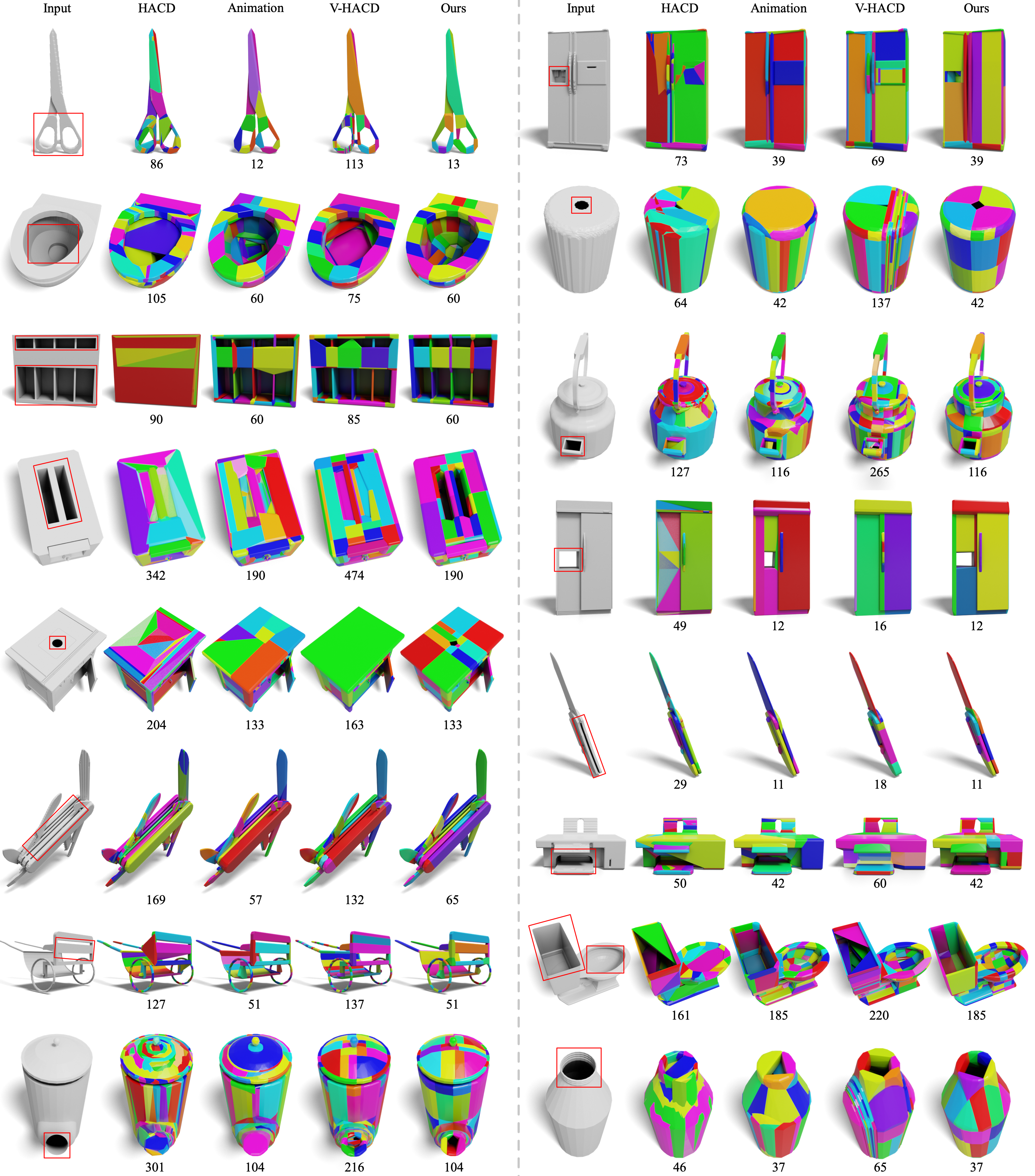
An image from the CoACD paper comparing CoACD (“Ours”) with existing methods.
I have already started porting CoACD to Rust! Right now, I have implemented just the mesh cutting algorithm, which is rather cool by itself:
Remaining work includes things like the concavity calculation, a Monte Carlo tree search for finding optimal cutting planes, and component merging. Hopefully I can get these working soon enough!
New Joint Solver
For several consecutive releases in a row, we have been meaning to rework joint APIs, change XPBD to another joint solver, and implement missing features such as joint motors. Avian 0.4 finally addressed some of these with the addition of joint frames and various other improvements, but the new joint solver remains unfinished, and motors are still missing.
A partial reason for this is that amidst me working on an impulse-based joint solver, AVBD (Augmented Vertex Block Descent) was published, catching seemingly the whole physics simulation community’s attention.
I had a basic 2D version implemented within just a few days (but had people informing me about it for weeks haha), to test out how well it works in practice. In short, my first impressions were unfortunately a bit of a mixed bag.
Pros:
- AVBD does handle both high mass ratios and high stiffness ratios quite well, as advertised.
- The vertex coloring in AVBD provides superior parallelism compared to the typical edge coloring used by dual solvers. Great for GPU physics and multi-core CPUs!
- Especially for joints, AVBD seems really impressive in my testing. Even complicated scenarios have very little stretching or high-frequency oscillation.
Cons:
- Despite what the AVBD paper likes to say, the parameters are really fiddly and scene-dependent. Tuning is required for good behavior.
- The above can be somewhat mitigated using a post-stabilization step, but in my experience, this can make stability even worse.
- The body solve order has a significant impact on results. Without shuffling the order, joint chains can exhibit clear visual artifacts that depend on the iteration count.
- Using wide SIMD seems more difficult for the primal update than it is with dual solvers, which hurts CPU perf and single-threaded use. Game physics rarely runs on the GPU.
- The soft constraint formulation of impulse-based constraints provide a frequency and damping ratio for tuning constraints, while AVBD just provides a mass-dependent stiffness
k, which is a nuisance for game designers. See Soft Constraints by Erin Catto. - Speculative collisions and joint limits seem more challenging with a position-based solver, though it’s probably doable.
- The Hessian math can get seriously complicated for many 3D joints, and is often fairly expensive unless you’re willing to make approximations at the cost of some stability.
- Regardless of tuning, for contact scenarios, I was struggling to get results that were even close to being as stable as our existing TGS_Soft (aka “soft step”) solver.
- AVBD breaks Newton’s third law. When bodies A and B collide, the force applied to A is not necessarily equal or opposite to the force applied to B. It is generally close enough, but it just means that this is one fewer invariant you can rely on.
(To emphasize: these are just my own experiences from experimenting with AVBD for a few weeks, and trying out the author’s demos. Your mileage may vary!)
What AVBD accomplishes is extremely impressive, and there are certainly cases where it shines and is a great fit (ex: GPU physics). However, for general-purpose game physics on the CPU, I am not yet convinced it is the best fit. If some of the stability and tuning issues can be addressed, my view on this may change, but for now, I am still leaning towards a traditional impulse-based solver for Avian’s joints.
For cases where impulse-based joints struggle, such as high mass ratios, we could implement a reduced-coordinates multi-body joint solver such as the one in Rapier. This is also the approach taken by engines like PhysX and Havok.
I may still keep experimenting with AVBD though, and am interested to see how it develops!
Support Me
While Avian will always be free and permissively licensed, developing and maintaining it takes a lot of time and effort.
If you find my work valuable, consider supporting me through GitHub Sponsors. This is ultimately my hobby, but by supporting me you can help make it more sustainable.
Thank you ❤️